World’s Biggest Distributed Representations…
and how to handle them. The original champions of distributed processing, the connectionists, have faced just this issue. Many connectionist models feature hidden layers in which localist interpretation breaks down. (Whence all the bruhaha about distributed processing.) When localism fails, connectionists turn to multivariate statistics for help. A variety of analytical techniques all work to reduce the dimensionality of a target domain. Suppose, for example, we want to understand the various patterns of activation of a hidden layer of eighty units. Multivariate thinking begins with a simple conceptual shift: Regard each activation value as a magnitude along an axis or “dimension.” Eighty units, in this way of thinking, represent a space of eighty dimensions, and the eighty activation values are interpreted as coordinates in that space. In other words, the pattern of activation with its eighty coordinates is reconceived as a single point in 80-d space. This 80-d space is thus a handy container for many patterns of activation — each reappears as a specific point in a high-dimensional map.
At this point the analysis proper begins: An 80-d map is not something we can look at, but it is definitely something whose geometry we can measure. No matter how high the dimensionality, the notion of distance between points can retain its usual non-boggling one-dimensional sense. Euclidean (linear) distance between any two points is easy to calculate, or one may calculate similarity between points with many other algorithms. The result is a matrix of distances (or dissimilarities), not unlike a matrix of mileages between cities. Having extracted the distance matrix from the 80-d mapping, it is now possible to survey and interpret the activation space via several different techniques, each of which can reveal aspects of the structure of the galaxy of points in activation space. One appealing analysis of this type is multidimensional scaling (MDS). MDS uses the distance matrix from points in a high-d space to build a new mapping in a space of fewer dimensions. The MDS condensate can be of arbitrary dimensionality. In choosing the degree of shrinkage, one faces a tradeoff between accessibility and accuracy of the resulting low-d map. More dimensions afford a better fit between the new map and the actual distances, but remain hard to interpret, while fewer dimensions (two or three) are easy to visualize but, depending on the data, could be too procrustean, yielding a new map that wildly misplaces points. One sets the balance of accessibility and accuracy according to taste.
Let us suppose that our 80 unit hidden layer computes 80 functions in a completely localized, modular way; that is, each unit specializes in one function, and is active only when the network computes that function, and inactive otherwise. (For this example, assume that units are either on or off, 1 or 0 in activation value.) In that case, the 80-d activation space is studded with points that lie exactly on its 80 axes, each orthogonal to all the others. If we were to attempt MDS analysis of this space, we would encounter a double disappointment. First, as we shrunk the dimensionality of the space, we would be forcing points on orthogonal axes onto single new axes, resulting in a very bad fit, ever worse as the amount of shrinkage increases. Second, the activation space would be without structure. That is, every point is equidistant from every other. Any grouping of points will be completely arbitrary, not supported by underlying order in the space.
Now let us suppose that the hidden layer is a sparsely distributed processor. In this case, a subset of units work together to compute each function, and these subsets partially overlap from function to function. If we scale this space to fewer dimensions, the overlap means that axes can coalesce without as much forcing, and that the overlaps might reveal a meaningful structure in activation space. That is, where we judge two functions to be antecedently similar, we may expect the activation space to somehow reflect that similarity, and our new MDS’d map to reveal some of that structure.
Over the last two years I’ve been focusing the lens of MDS on the accumulated PET studies in Brainmap and in the PET literature in general. My goal has been to use MDS as a crude probe of brain activation space. If MDS works without excessive procrustean stress, and if the structures detected by MDS are meaningful, this will offer another line of evidence that the brain is indeed a distributed processor.
As with any meta-analysis, this approach requires careful registration of the original experimental observations in a common format. The PET studies themselves already encourage comparisons in many ways. Individual brains differ strikingly in size and shape, so a routine part of PET processing is the morphing of one’s personal brain into the shape of a standard brain, so that points of activation can be localized to comparable anatomical structures. In addition, PET studies always involve multiple subjects. The resulting patterns of activation are averaged (and peaks tested for significance), washing out stray activations, whether due to idiosyncrasy or to a subject’s straying off the task. Beyond that, however, the studies differ from one another in one important way: As mentioned above, the reported patterns of activation are generally “difference images,” created by subtracting a baseline or control pattern from the test or task pattern. These baseline controls are not uniform in the literature. For example, in a study of semantic processing, study A might image a brain during reading aloud, and subtract from that a control task consisting of reciting the alphabet. The point of this subtraction would be to isolate the subsystem involved in processing word meaning, while factoring out that involved in simple vocalizing. Study B, meanwhile, might also image a brain during reading aloud — the same test task — but subtract from it a control task consisting of reading silently. In this case, the function of interest is vocalizing itself. Both studies might display patterns of activation labelled “reading aloud,” and indeed the underlying activation in the brains involved might be very similar, but the divergent subtracted control states would yield divergent difference images.
As a result, any PET meta-analysis must rest on a collection of experiments that share a common control state. There are a few such familiar baselines in the literature. One of the most common baselines is simple rest with closed eyes. A full review of hundreds of PET papers yielded 36 experiments where the difference image was based on a control state where subjects rested quietly with eyes closed. (Another common control condition has open-eyed subjects focus on a fixation point on a blank screen. This will be reviewed in a future study.) In these 36 experiments, points of activation were assigned using a brain atlas (as well as published anatomical assignments) to approximately 50 discrete brain areas, chosen to minimize overlaps and thereby minimize double-counting of points of activation. To wax multivariate, individual patterns of activation in the brain were conceived as points in a 50 dimensional space. From here, multi-dimensional scaling generated maps in fewer dimensions. Surprisingly, the procrustean stress, or badness of fit, was quite low even at 3 dimensions.
MDS did reveal the crude outlines of the structure of brain activation space. The largest regional affinities in brain space were determined by the modality of input. Tactile, visual, auditory, and no input conditions tended to group. The groupings were not compact clusters, however, but rather rough ellipsoids. In other words, in many cases similarity of input modality leads to collinearity of resulting points in brain activation space. Within the modalities, there is some indication of further structure, and this seems to be in part a reflection of the response made to the various tasks in the map.
The figures below reveal this collinearity and internal structure. Each is a view through a 3-dimensional MDS space, based on the 36 experimental points in 110 dimensions. The figures are paired, showing two views of the same set of points. The first view rotates the space so that the ellipsoid space of points is seen from the end — what appears to be a tight cluster is in fact points deployed along an axis through brain space. Then in a companion figure the space is rotated to look at the point set from the side, displaying its internal structure. Each pair labels a different set of points. All 36 task points appear in each of the figures. However, a different subset is labelled in each pair, for ease of interpretation.
Only the relative position of points is meaningful; The XYZ axes are arbitrary. Nor do the positions of points bear any one-to-one relationship with anatomical or physical points in the brain. Each point represents an activation pattern of ten or more anatomical components, and point proximity indicates similarity among patterns. In short, the images that follow condense a large quantity of data — many experiments, many subjects. Here then is a first multivariate survey of “brain activation space,” and a brain-based window into the mind.
Figure 1A: Tasks with no stimuli, showing their collinearity.
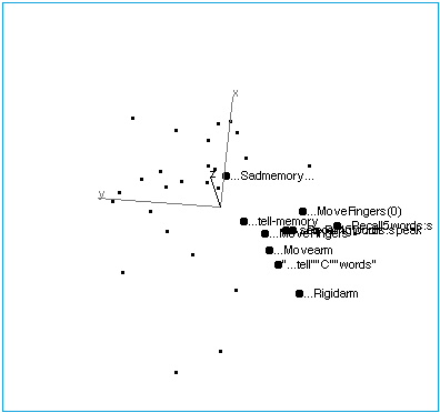
Figure 1B: Tasks with no stimuli. The space has been rotated to reveal the internal structure of this region of brain space. The following labelling conventions apply to all figures: Each point label includes capsule information about stimulus, task (instructions given to subjects before the scan), and response. Ellipses (…) indicate no stimulus when they lead the label. In this region of brain activation space, tasks that involve limb movement group at one end of the no-stimulus axis, while tasks that involve memory and spoken response lie at the other end. “…Sadmemory…” falls off the axis — in this task, subjects were asked merely to recall a sad scene, but make no physical response.
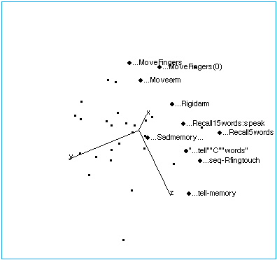
Figure 2A: Audition. A rotation of brain activation space to reveal the collinearity of tasks with auditory input.
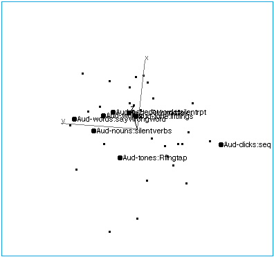
Figure 2B: Audition. The space has been rotated to reveal the structure of the auditory axis. At one end, points are characterized by verbal inputs and outputs, although actual speech (vs. imagined speech) does not seem to affect placement. At the other end of the axis are tasks involving nonverbal auditory stimuli, and nonverbal responses.

Figure 3A: Tactile stimuli. Space rotated to indicate rough collinearity along the axis of tasks with tactile input. R and L indicated Right and Left, respectively. “Tesoph” — tactile stimulation of the esophagus.

Figure 3B: Tactile stimuli. The rough structure of the tactile axis. Stimuli to either hand seem to group, as do stimuli to the esophagus and to the toes. Further from the group lies a task wherein subjects explore a solid object and indicate with a “thumbs up” if it is a parallelopiped.

Figure 4A: Vision. Indicating the limited axis collinearity of five visual tasks.
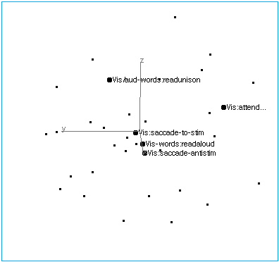
Figure 4B: Vision. Structure of the visual axis. Simple visual inputs and saccadic responses group, as do verbal stimuli/responses. A visual attention task lies off the axis.

Figure 5A: Verbal responses. The space in this figure is oriented as in Figure 4B. Note that the type of response is not a salient organizing principle of brain activation space. Here, all the verbal response tasks are shown, but they exhibit neither collinearity nor other obvious affinity.

Figure 5B: Verbal responses. As in 6A, but rotated for ease of reading.

Figure 6A: Motor responses. As with verbal responses, tasks requiring a motor response do not exhibit salient structure in brain activation space. (Space is oriented as in 5B.)
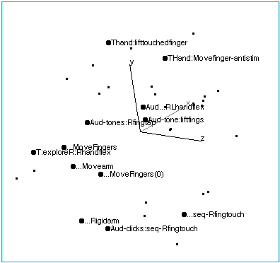
Figure 6B: Motor responses. As in 7A, rotation reveals no collinearity nor other grouping.

These images are static. To fully explore brainspace, it may be helpful to climb aboard the shuttle and pilot yourself through the heart of it. The same data depicted above have also been plotted in a virtual universe that you may visit. The file, filename*, is written in VRML 2.0 (“Virtual Reality Modelling Language”). Your browser may need to be equipped with a plug-in to handle VRML. An excellent one, available for both Mac and Windows, is cosmoplayer.
Therefore… (From these observations follow some tentative conclusions about the nature of consciousness).