Dan Lloyd, Department of Philosophy and Program in Neuroscience, Trinity College, Hartford, CT 06106
Email: dan.lloyd@trincoll.edu
Draft of 1/13/07
Abstract: This hypertext reports on a meta-analysis of 478 published fMRI studies (whose results have been archived at www.brainmap.org), to address the issue of functional localization: Do individual regions of the brain have limited, specific, and dedicated functional roles in cognition? Or conversely, are distinct cognitive, perceptual, or motor tasks supported by exclusive regions or groups of regions (“networks”) in the brain? The outline just below links to main sections of the methodology, results, and discussion. The text below that is the full rationale for the study, its methods, and its conclusions. Indents signal subordinate argument or explanation, which can be skipped for a quick first read.
This is a work in progress; I hope for a steady state by Spring 2007.
Outline:
- The issue: Are particular brain regions dedicated to particular cognitive functions?
- Casting a broad net: 10,000 brains
- Results: Brodmann x function — the data tables
- Drilling down: 386 anatomical areas x function (in progress)
- Visualizations (in progress)
- Main conclusions from the study (in progress)
The issue: Are particular brain regions dedicated to particular cognitive functions?
 Cognitive neuroscience is committed to fusion of mind and brain under the concept of the neurocracy: the whole mind is the sum of the actions of myriad brainy parts. But “neurocracy” is ambiguous. It echoes “bureaucracy,” and much thinking in this field assumes and justifies a bureaucratic frame for mind-brain unity. In the neurocracy (under this reading), neurocrats are assigned highly specific and quite stupid jobs to perform; each neurocrat has one or perhaps a few functions. The intelligence of the whole, then, is the result of the careful design of the workflow in the neurocracy: Low level neurocrats pass useful memos down the line to other neurocrats who know how to merge them into executive summaries. Eventually the last departments of the neurocracy issue orders to the muscles, laws to the other departments, and decrees to the world.
But “neurocracy” equally echoes “democracy.” Instead of neurocrats of specific and limited function, neural citizens all share the responsibility of government. Each does its best to follow the news, and vote according to its preferences. Despite their limited expertise, from moment to moment low level agents don different functions, mobbing one issue after another; the neurocracy (under this reading) is not so much a warren of cubicles as a suite of meeting rooms. The behavior of the whole organism, then, is the result of a million polls a minute.
Which is the human brain? Neurobureaucracy or neurodemocracy? To the extent that the brain is a bureaucracy, what are its main anatomical departments and what is the job of each? These are the questions explored here.
Neurocracy, in either case, explains high level minding (complex behavior, intelligence, consciousness) as the synthesis of lower level braining (channels, synapses, circuits, networks, areas…). As a philosophical issue, any bureaucracy can be reconstrued as a democracy, depending on how big the whatever-crats are or how broadly their functions are described. But there’s an empirical version. Science has at hand established entities on both the mind and the brain side, and the neurocracy question can be raised about them. Minding is of course the province of psychology, and among its many taxonomies we will look here at a standard outline of cognitive and perceptual operations in the domains of action, cognition (including language), emotion, and perception, with subtypes under each. Meanwhile, the brain can be anatomized at levels from molecules up to hemispheres. Here we focus on the high level geography afforded by functional Magnetic Resonance Imaging, fMRI. Even at this level, the map is layered with the history of neuroanatomy. One common schematic carves the cortex into Brodmann Areas, based on the painstaking histology of Korbinian Brodmann almost exactly a century ago. Brodmann mapped the cortex according to types of neurons and their density in different cortical layers. The areas he numbered (1 to 52 in each hemisphere) followed the variations in the cellular architectures he observed. No doubt Brodmann’s map will need some re-districting, but, absent a consensus on just what the parts of the cortex “really” are, the Brodmann areas (BAs) enjoy the weight of tradition. Functional MRI studies will almost always refer their findings to the BA map, providing a steady basis for comparison across experiments.
So from the vague question of neurocracy we can extract a more exact version, namely: Are the Brodmann Areas bureaucrats or democrats? Or: Does each BA have one or more specific functions to perform, or does each contribute to a broad array of functions? The same issue can be raised from the other end: Are specific cognitive/perceptual/motor functions implemented in specific areas? These are the questions of functional localization, and the neurobureaucracy is a realm of localization. The neurodemocracy, in contrast, supports the mind by distributing functions over a number of areas.
Of course, there is no all or nothing answer. Between the bureau- and the demo- interpretations one finds a spectrum of intermediate cases. Some BAs might be quite specific in their jobs, while others are generalists, or perhaps all fall into an in-between camp of partial specialization. In any case, the functional leanings (if any) of the separate Brodmann Areas will be an important piece of the big picture of the brain, and contribute to the ongoing story of the integration of the mind with its neural substrate. But the overall question is also important, because to a large extent functional brain imaging studies are designed with the neurobureaucracy in mind. Taken one by one, they often presuppose localization of function. (Not all studies, but many.) If the brain in general is bureaucratically organized then this presupposition is harmless. But if there are many examples of distributed function, then we have to think about tilting experimental designs to discover these, or revising interpretive strategies.
Casting a broad net: 10,000 brains
The contrastive strategy and its limits
The typical brain imaging experiment compares one or more experimental conditions to one or more control conditions, with appropriate attention to a variety of potential confounds and sources of “noise” (more on this below). For example, suppose we want to know if particular areas of the brain are specialized for recognizing faces. This is a straightforward neurocratic question: Is there a brainy neuocrat with the narrow specialty of faces? Or is face recognition assigned to a committee of neurocrats, each bringing a relevant skill to a working group assembled when faces are need to be recognized? You might think that this is easy to test: Put a volunteer in the scanner, show her some faces, and look at see if any areas “light up.” Unfortunately, it isn’t so simple. The “raw” signal from fMRI will show a signal from the whole brain, a mottled, jiggling furor that extends from end to end, lobe to lobe. That’s because the scanner detects metabolic activity (usually, the contrast between oxygenated and deoxygenated blood, the “Blood Oxygen Level Dependent” (BOLD) response); you would expect and fervently hope that such activity appears in the neighborhood of every neuron. The metabolism-based signal, then, is mixed with a great deal of noise; noise swamps signal about 100 to 1. So maybe your image is showing some specialized face-detection in some areas of the brain, but you’ll never be able to see it just by looking.
A frequent workaround to the noise problem is to set up a contrast between many images (averaged together) taken in two separate conditions. In this case, we’d get images of you looking at faces, and images at you looking at something else (or nothing), and look for the differences in the brain while looking at faces. In the contrast image resulting from this subtraction the global metabolic jiggle and the incessant static would pretty much disappear, since those are constant concomitants whether you’re looking at faces or not. The leftover, then, should be the added activity that is specific to the processing of faces. In brain imaging research, it is these leftover contrasts that are depicted as blobby hotspots in the colorful graphics that accompany every research report.
The contrastive approach rests on some controversial assumptions, and in practice it is not as simplistic as I’ve described it. Nonetheless, it is the approach taken in the experiments reviewed in this analysis. The results of contrastive experiments are precisely recorded as peaks of activation, the hottest and brightest points in the blobs. The experiments here reported from one to 31 of these local maxima, with an average of around 7 peaks per experiment. Thus, there are two ways to display results: as a sheaf of contrast images or as a table identifying the local peaks of metabolic activity. In a table, under each experiment you’d list the xyz coordinates of each peak (each blob center) and the anatomical names of its region (including the Brodmann Area number), along with measures of the extent and intensity of the activation.
This science shares with all science the goal of rising from particular observations to generalizations, good bets about what you’d observe in further tests in similar conditions. Every experimental report is already a compilation of repeated observations during many trials by multiple subjects. Refining the statistical power of neuroimaging is a continuing task shared by a large research community. So, if our notional face experiment reports that face recognition is associated with activity in the fusiform gyrus (BA 37), then this association should be regarded as a reliable piece in the big picture of the neurocracy.
Nonetheless, the contrastive approach stumbles exactly on the problem posed here, the question of neurocracy.
 A schematic example can illustrate the problem. Suppose that our analysis of some cognitive capacity suggests that it comprises component functions A, B, and C, and these are implemented by some unknown combination of just three regions in a (small) brain. Further suppose that the exclusivity assumption is violated, and that the functions are implemented in overlapping brain regions: A depends on areas 1 and 2; B depends on areas 1 and 3; C depends on areas 2 and 3. These are the stipulated facts of the scenario. Will subtractive “brain imaging” be able to discover them? Following the subtractive recipe, we collect and average “raw” images during each of the three tasks, and derive the contrasts. Here is the full list of possible outcomes:
A(1,2) – B(1,3) = region 2
A(1,2) – C(2,3) = region 1
B(1,3)– A(1,2) = region 3
B(1,3) – C(2,3) = region 1
C(2,3) – A(1,2) = region 3
C(2,3) – B(1,3) = region 2
The math is strange, in part because only positive values are kept in typical image subtractions. (A-B, for example, leaves behind not only region 2, but a “deactivation” of 3.) More important, the results are empirically wrong in the scenario: None of the possible subtractions correctly identify the regions involved. Two experiments about function A could yield contradictory results, yet both would be correct. Nor does it help to contrast A with the conjunction of B and C, despite the appearance that this would sharpen the result (the function vs. everything else). In this case, A – (B &C) excludes all of the areas supporting A. In short, when functions overlap in their implementations in the brain, the strong conclusion that a contrast image shows the areas dedicated to the function is invalid. What can be concluded is that the revealed areas are part of the implementation, but that none of the other areas can be excluded. That is, the neurocracy question is unanswerable through any single contrast.
Contemporary cognitive neuroscience is far more sophisticated than this caricature of the contrastive method suggests, of course, and researchers are responsive to the problems of interpretation. Here, however, I propose to explore another way to cast the net, and make use of contrastive experiments to address the nonsubtractable issues of neurocracy.
The small brain example suggests two strategies for overcoming the limitations of individual contrasts. Both depend on increasing the variety of contrasts considered: First, we could begin with a brain region and consider all the contrasts that activate it. In the schematic example, region 1 was the residue of two contrasts, two notional “tasks.” Separately, neither contrast correctly identified the disjunctive function of the region, but taken together they correctly identified hypothetical functions A and B. In general, then, a “brain first” strategy works region by region through the brain, and identifies all the contrasts that “light up” that region. Collectively, the disjunction of all the functions targeted by these region-specific contrasts characterizes the overall function of the region more completely than any single contrast.
Second, we could begin with a function and collect all the contrasts that use tasks that implicate the function. In effect, a “function first” strategy diversifies the base-line conditions by which the contrast is measured. In the example, two contrasts probe function A, extracting two different contrastive functions. Neither of those contrasts completely identified the involved brain regions in the function, but conjointly they do correctly indicate regions 1 and 2.
The small brain example affords a complete reduction of function to region(s) by expanding and diversifying contrasts, and grouping them by region (the brain-first strategy) or by function (the function-first strategy). They illuminate a conceptual shift that occurs when distributed processing is a possibility. If modularity is assumed, then the various contrasts possible in the small brain data are inconsistent, and as a result the inconsistency must be explained away by further elaborations in the interpretation of the diverging results. Many discussion sections in this literature do exactly that. But in the non-modular framework, the apparent inconsistency is the predicted effect of diverging target or baseline tasks in various experiments. Differing contrast results triangulate the underlying distributed function. In this way of thinking, the discrepancy is itself the positive evidence for the underlying distributed processing. It doesn’t need to be explained away. (However, if two experiments use the same target and baseline tasks, then their results should agree, just as individual subject results within one experiment should agree.)
The smallness of the example makes the two strategies look easy, but the net must be cast widely to overcome the illusion of exclusivity. In principle, every neuroimaging experiment yields results that constrain every cognitive function, as well as the function of every area of the brain. With thousands of studies in print, this is a tall order. Fortunately, however, several visionary researchers have seen the need for synoptic databases that compile the results of many imaging studies. One of these databases is Brainmap, created by Peter Fox and Jack Lancaster, and maintained with a web interface at the University of Texas at San Antonio. Brainmap records the loci of peaks of activation revealed by experiments using various experimental strategies, along with brief descriptions of the experiment, citation details, the subject groups, the imaging modality, and the type of cognitive function probed. That is, it condenses many published results in functional brain imaging. (Another ambitious archive, the fMRI Data Center, offers summary data along with the raw image data itself, pixel-by-pixel. See http://www.fmridc.org/f/fmridc.) As of January 2007, Brainmap archived 959 papers reporting 4,221 different experiments. Collectively, this body of research reports 34,223 significant peaks of activation.
Brainmap records most of the relevant conditions and results for each paper archived, including the locations of peaks of activitation. The database is searchable by anatomical area, region of interest, task paradigm, behavioral domain, and many other categories of interest. For this study, I looked at 37 behavioral domains. They’re listed below, with the number of experiments reported for each.
| Action.Execution | 67 |
| Action.Execution.Speech | 4 |
| Action.Imagination | 6 |
| Action.Inhibition | 19 |
| Action.Motor Learning | 1 |
| Action.Observation | 9 |
| Cognition | 33 |
| Cognition.Attention | 173 |
| Cognition.Language | 11 |
| Cognition.Language.Orthography | 37 |
| Cognition.Language.Phonology | 37 |
| Cognition.Language.Semantics | 107 |
| Cognition.Language.Speech | 44 |
| Cognition.Language.Syntax | 11 |
| Cognition.Memory.Explicit | 37 |
| Cognition.Memory.Working | 143 |
| Cognition.Music | 6 |
| Cognition.Reasoning | 17 |
| Cognition.Space | 24 |
| Cognition.Time | 1 |
| Emotion | 32 |
| Emotion.Anger | 2 |
| Emotion.Anxiety | 1 |
| Emotion.Disgust | 16 |
| Emotion.Fear | 11 |
| Emotion.Happiness | 14 |
| Emotion.Sadness | 11 |
| Interoception.Hunger | 2 |
| Interoception.Sexuality | 3 |
| Perception.Audition | 44 |
| Perception.Olfaction | 3 |
| Perception.Somesthesis | 134 |
| Perception.Somesthesis.Pain | 26 |
| Perception.Vision | 28 |
| Perception.Vision.Color | 4 |
| Perception.Vision.Motion | 74 |
| Perception.Vision.Shape | 57 |
As authors deposit their data in Brainmap, they categorize each experiment under one or more of these domains. (In a separate study, researchers established that these categories are used consistently by the large community of contributing researchers.) As you can tell by the numbers, the super catagories “Emotion” and “Cognition” do not combine all their subtypes. Rather, they function like “other” or “none of the above.”
The database currently records 4250 experiments; this review used “only” 1249 of them. That’s partly due to the closing date of this review, early summer 2006. More studies have been entered into the archive since. More important, the studies used were filtered with the following criteria. The experiments in play are all:
- fMRI studies
- normal subject experiments (i.e. excluding patient groups, children, seniors, special subpopulations like musicians, for example. Experiments separating male and female results were included if both were available.)
- “Main effects” (i.e. positive activations, the experimental result of the contrast between the task and a control condition. Accordingly, the review excludes published meta-analyses, probes of modulatory effects, parametric studies, and any experiments where it wasn’t clear that loci were main effects.)
Also, each experiment was reviewed to confirm that the target task would typically be assigned to the target domain, considered in contrast to its control tasks. This led to a few adjustments, and in cases of lingering uncertainty, omission of a few experiments.
Here then are some results:
Table 1.0, hits in all behavior domains compared with all Brodmann Areas (all BAs, that is, that recorded any activity in any experiment). BAs are separated by hemisphere (L and R). Sub- lobar regions are collected in a single bin, “L” or “R” with no attached number. Each hit in a BA means that one experiment reported at least one peak of activity in that BA. So values in each table cell record how many experiments found activity in each BA, within the domain of the experiment.
But there is a problem: In general, we want to avoid a misleading base rate fallacy. In this case, one could greatly exaggerate the contribution of a BA area to a particular domain. For example, from Table 1.0, one would conclude that area 6 is massively dedicated to attention tasks, because about 70 attention experiments provoked activity in this region. But that appearance is largely due to the fact that very many experiments happen to be attention experiments, or in other words that the base rate of samples (experiments) is high, compared to other domains. For that reason alone any area involved in attention will seem to be mainly involved in attention. Meanwhile, just one experiment targeted anxiety as its main effect, so its maximum possible cell score is 1. We fix this by “normalizing” the scores in each row, dividing all their values by the number of experiments probing that particular domain. So the hit counts under “Cognition. Attention” will each be divided by 173, the number of experiments in the domain. The cell values should now be interpreted differently; they represent the fraction of experiments in each domain that reported activity in each BA. This is recorded in…
Table 1.1, fraction of reported experiments that record hits in each domain, compared with Brodmann Areas. That is, reported hits normalized by number of experiments in each domain. Each domain (row) label links to a graphic version of the row, indicating the score for that domain in each BA. Each BA label (the column headings) links to a graphic showing the domains involved. (Note that this may still be under construction.)
At some point, you may want to know the bibliographic sources for the tables. You’ll need:
Table 0.0, Brainmap reference numbers for experiments in each domain. The main number in each listing, e.g. 3054, is the Brainmap paper reference number. At the Brainmap website you can use that number to search for the full records for each paper (http://www.brainmap.org). Or you can click on this reference number and jump to the PubMed abstract. Typically, each paper will report on several experiments, of which some were candidates for this review. So, in Table 0.0, the paper reference number will be followed by one or more experiment numbers. For example, 3054.2, 3, 4 signifies that in paper 3054 I harvested points from experiments 2, 3, and 4. This numbering follows Brainmap as well. (Note that some papers involved experiments in multiple domains; these are listed redundantly in each domain in which they occur.)
But there is another problem: Table 1.1 corrected for the disparities in the number of experiments pursuing the various behavioral domains. There is a similar problem posed by promiscuous Brodmann areas. Area 32, for example, turns on for 24-26 domains (R-L). So the claim of any domain that it is especially implemented in Area 32 will be disputed by two dozen other domains. But lonesome Area 33 (Right) responds in just one condition, in the domain “Interoception, sexuality.” (Perhaps “lonesome” is the wrong term.) Sexuality also excites 21 other areas, but those are all active for other domains as well. Intuitively, that single arousal of BA 33 seems weightier in its unique attachment to a single domain, in contrast to other areas that seem to serve many domains. So we normalize again, this time to discount the BAs that are exceptionally busy and amplify those that support just a few domains. This revision leads to Table 1.2, Brodmann areas involved in various domains, normalized by domain and area base rates.
But is this last adjustment warranted? If one BA is serving many domains, and another is serving few, why should the former be discounted in its contribution? If we’re looking at the spread of BAs involved in a behavioral domain, should it matter that some are involved in other domains and some are not? One’s answer depends on a further elaboration of the neurocracy issue, namely, the meaning of “neurodemocracy” — distributed processing. For example, consider again Area 32, active in about two thirds of all domains (119 experiments found activity in R 32, 143 in L 32). With respect to the 37 domains, BA 32 is clearly no narrow bureaucrat. But there are two ways to think about its actual function. It might be a substrate for all its domains, performing one process which is implicated in all of them. Or it might be an alternator, switching its processing as needed. Or, as always, it might be some mix of both. How you balance the numbers depends on this issue: If BA 32 is a substrate, then its contribution to any domain is not uniquely different from its contribution to other domains. In that case, it plays a lesser role in explaining the neural differences behind the domains. So it should be discounted (though not discarded), leading to the normalization by BA base rate, Table 1.2. On the other hand, if it is an alternator, then it really is doing something different in each domain. It is as if it were a different area in each domain. In that case, its role can’t be slighted in comparison to that of other, less versatile, areas. Table 1.1 would not need further normalization.
In this analysis, we opt for the substrate reading (and Table 1.2), but you can make your own call. That’s why so many tables are attached. You can choose the one you find most legitimate, download it, and dig in. Arguably, either Table 1.1 or 1.2 need no further adjusting. After all, each data point represents a published, significant finding based on multiple subjects, published in a peer reviewed journal. The tables simply put many such studies together. If you are interested in a descriptive summary of experiments in a particular behavioral domain (= one row), or in a descriptive summary of experiments engaging one Brodmann area (= one column), then these tables are all you need.
And, at this point, we can outline an answer to the neurocracy question: In general, overall support of the behavioral domains is highly distributed. On average, forty (of 86) Brodmann areas are involved in each domain. More specifically, as the number of experiments in a domain increases, the number of BAs discovered to be involved also increases. But as the experiments pile on, there seems to be a rough upper limit to the number of areas involved, at around 55 BAs. (Here is a graph plotting number of experiments against number of BAs with activity.) The asymptote of the trend line is about 55.) Similarly, each Brodmann area is highly versatile in its support of varying behaviors. On average, each area is involved in 17 (of 37) domains. Bear in mind, too, that each datapoint is the result of a contrast that has already subtracted out part of the neural support for the function under study. In terms of cerebral cortex, as carved by Brodmann, it takes extra effort by more than 40% of the brain to do anything. Conversely, the typical Brodmann area is differentially engaged in 40% of behavioral (cognitive, perceptual, emotive) domains. Even if these percentages are blurred (as no doubt they are), the sheer numbers of the meta-analysis are apparently trending toward neurodemocracy.
But there is another problem, a hangover from the base rate problems above. The neurocracy issue is inherently comparative. The overall characterization of BAs and functional domains (just above) is suggestive, but vague. The more specific issue would concern particular functions or particular brain areas. As always, some functions are localized, and some brain areas are specialists, but which ones? Individual contrasts can’t resolve the specifics, for the reasons above. But a huge meta-analysis allows us to embed and compare particulars in a brain-wide and function-deep context. This leads to a new set of problems, however, a nasty hangover from the baserate issues corrected above. This is the problem of multiple comparisons.
Nothing is ever certain, of course. Individual hypotheses in science are conventionally confirmed with 95% (or better) confidence. (Strictly, that is a 95% confidence that the null hypothesis is false.) Conversely, each hypothesis runs a risk, up to 5%, of being spurious, due to chance alone. So as more experiments pile up concerning any particular hypothesis, the chances of one among them turning in a false positive increase. Our meta-analysis of 8179 particular hypotheses may have as many as 400 mistakes due to pure chance, and we would surely like to eliminate these. We must raise the bar by setting a threshold for admittance into the big table of results. But how is that threshold to be set?
For present purposes, we’ll do this globally, which is to take a rather blunt instrument to the data. That is, the result is likely to be over restrictive, omitting observations that are significant. We’ll calculate the confidence interval around the mean of values in Table 1.2, and preserve the data that exceeds a .05 level, subject to a correction for multiple comparisons. (In this case, a “Bonferroni correction.”) The correction will, in effect, lower the critical threshold to allow for the possibility that amid the large collection of observations, some of them are due to chance. This leads to Table 1.3, Significant relationships between areas and domains, normalized and corrected for multiple comparisons. The table is simply the values of Table 1.2, each divided by the global confidence threshold, keeping only those values greater than 1 (i.e., greater than the threshold).
With respect to the neurocracy, this thresholding approximately halves the totals above. On average, each domain is supported by 22 Brodmann areas; Each BA supports around 10 domains. That’s about 25% in both directions — still rather democratic and distributed.
From here, the analysis turns more specific, and is currently in progress. For now, the final table tries to make the results so far legible without eyestrain. Table 1.4, Summary of Domain by BA activity, flags each hit with the BA number. You can look across each row and see it as a list of BA numbers, with right on the left, as in all the other tables. (This R-L reversal is an unfortunate consequence of some earlier computations.)
It looks like this:
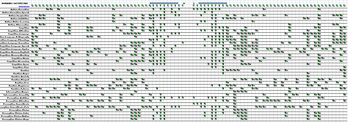
(to be continued….)