Terra Cognita: From functional neuroimaging to the map of the mind
Draft of June 15, 1999
(Brain and Mind, 1: 1-24, 2000. )
Dan Lloyd
Department of Philosophy and Program in Neuroscience
Trinity College
Hartford, CT 06106
dan.lloyd@trincoll.edu
Abstract
For more than a century the paradigm governing cognitive neuroscience has been modular and localist. Contemporary research in functional brain imaging generally assumes this modularity in its quest to localize particular functions in one or more specific brain regions. Meanwhile, connectionist cognitive scientists have celebrated the computational powers of distributed processing, and pioneered methods for interpreting distributed representations. This paper takes a connectionist approach to functional neuroimaging. A tabulation of 35 PET (positron emission tomography) experiments strongly indicates distributed function for at least the “medium sized” anatomical units, the cortical Brodmann areas. More important, when these PET experiments were interpreted as distributed representations, multidimensional scaling revealed a “brain activation space” with a salient structure organized primarily by the sensory modality of the stimulus, and secondarily by the type of motor response. These results suggest that the localist paradigm should be augmented by distributed processing analyses, and that these analyses may lead to many discoveries about the structure of “inner space.”
Terra Cognita: From functional neuroimaging to the map of the mind
Is the human brain a parallel distributed processor? To many cognitive scientists and philosophers, the answer is a clear yes, possibly even a trivial one. In its support, cognitive science appeals to a double analogy. First, at the cognitive level, connectionist systems look like little brains in competence and performance. Computation spread out over a parallel network of relatively simple “units” offers a familiar menu of folksy features: plausible models of learning, sensible handling of novelty, sensible and spontaneous generalization, graceful degradation, fault tolerance, and others. In specific applications, connectionist models spontaneously develop some surprising analogies with human cognition (e.g. Rumelhart and McClelland’s reproduction of childrens’ errors in past tense production). Second, connectionists also celebrate the “neural inspiration” of their approach, pointing to resemblances between connections and synapses, processing units and neurons. So, at the implementation level, too, parallel distributed processors seem brainy. Taken together, this superficial similarity between biological brains and parallel distributed processing models, together with the many attractive cognition-like aspects of distributed processing, suggest that brains really are parallel distributed processors( McClelland & Rumelhart, 1986 , Rumelhart & McClelland, 1986).
Arguments by analogy are notoriously squishy, however, and obvious analogies are particularly suspect. We would hope eventually to cast aside the crutch of analogy, and pursue questions of neural computation directly, as empirical issues. In the literature of empirical cognitive neuroscience, however, the big idea of distributed processing rarely appears. Instead, at every level, we see continued adherence to the notion of local processing. The literature of cognitive neuroscience begins and ends with the hypothesis that anatomically identified brain parts have dedicated functions, and that the brain is an assembly of modular specialists.
In this paper I’m particularly concerned with localist hypotheses in functional brain imaging, especially Positron Emission Tomography (PET). Consider, for example, the following claims:
- Our results indicate localization of different codes in widely separated areas of the cerebral cortex (Petersen et al. 1988).
- These data localize the vigilance aspects of normal human attention to sensory stimuli…(Pardo et al. 1991).
- These experiments demonstrate the task dependence of visual processing, even for very closely related tasks, and the localization of the temporal comparison component involved in orientation discrimination in human area 19 (Dupont et al. 1993).
- The implications of these results are discussed, and it is argued that they are consistent with localization of a lexicon for spoken word recognition in the middle part of the left superior and middle temporal gyri, and a lexicon for written word recognition in the posterior part of the left middle temporal gyrus (Howard et al. 1992).
These are typical of the literature. (For a magisterial overview, see Posner & Raichle, 1994 .) PET methodology is mature and robust, so we need not question that the evidence supports each of the hypotheses above. But their general drift, the suggestion that the brain is a modular processor built of dedicated specialists, is false. To make this case, I exploit the abundance of PET literature, and its fortunate compilation in a massive database known as Brainmap, located at the Research Imaging Center at the University of Texas Health Science Center, San Antonio (ric.uthscsa.edu).
I. From local to distributed: a continuum
The distinction between local and distributed processing is, of course, not absolute. We might usefully mark the continuum of implementation with four subdivisions.
- First, to begin at the most localized, there could be networks of dedicated components. If the brain were a processor of this sort, anatomically defined regions would each be the sole locus of specific cognitively defined functions. This is modularity with a vengeance, radical compartmentalization of function.
- Second, there could be networks of dedicated (sub)networks. In the brain, one would expect to find subnetworks of multiple anatomically defined components, where each subnetwork is the sole site for specific cognitive functions. Although in this sort of brain a cognitive function is distributed over several regions, the processing is still localized insofar as each subnet is discrete. Although anatomically spread, the subnet as a whole is nonetheless a dedicated processor, uniquely charged with one job in the overall neural economy.
- Third, there could be sparsely distributed networks. Here anatomically defined brain regions are multifunctional. A region may be recruited to join a subnetwork to compute one function, and later recruited to a different subnet to compute a different function. Thus, subnetworks would overlap in their anatomy. This form of distribution is sparse, however, insofar as particular brain regions are not omnifunctional. That is, each function is computed by a subset of regions, rather than the whole brain. The engaged subnetworks overlap, but the adaptability of each region is limited to a fixed list of functions.
- Fourth, there could be fully distributed networks. Here every anatomically defined brain region has a part to play in every cognitive function, and no region is out of play. “Equipotentiality,” as Karl Lashley conceived it, is an early example of fully distributed processing.
The endpoints of this continuum are distinct, but the second and third options are open to an equivocation which is endemic in the PET literature: If one queries the brain about the location of a single function, or a few functions, one may discover a subnetwork correlated with that function, but it may not be possible to determine whether the subnetwork is a dedicated subnetwork, the “f system,” where f is the function under investigation, or whether the subnetwork correlated with that function is a snapshot of a sparsely distributed network in one of its many overlapping configurations. To resolve this ambiguity, one must shift from function-based research to component-based research. In other words, ask not “Where is this function computed?” Ask instead “What is this component doing?” If the majority of anatomically defined regions each handle just one or a few functions, some form of localization (including the specialized subnet version) will be supported. But if the majority of anatomically defined regions are each revealed to be multifunctional, this will support some version of distributed processing.
PET experiments abound. Their abundance invites a meta-analysis, and the flexibility of the Brainmap database affords exactly the questions just mentioned. To begin with some overview, Brainmap archives 733 distinct experiments (PET, MRI, and EEG), with a total count of local maxima of activation of 7508. That is a mean of 10.24 activation peaks per experiment. It is a rare experiment where all these peaks are located in a single region, suggesting distribution of function. But this in itself is not definitive, since the average experiment might just as well be picking out a dedicated subnetwork of 10 (plus or minus) components. A dedicated processor need not be packed into a single anatomical box.
A more decisive analysis would work through a list of components, asking of each whether it is a locus of activation for specific functions. Perhaps the narrowest anatomical specification of the brain accessible to PET discrimination is the cortical Brodmann area. Brodmann areas are distinct both in their geography and in their cytoarchitecture, two factors which indicated to Brodmann and generations to follow that each of these numbered areas were functionally distinct. Well, are they? The table below tabulates all of the reported areas of activation in thirty-five PET experiments. Thirty-eight Brodmann areas are involved, numbered along the top of the table. The thirty-five tasks explored in the experiments are encoded in condensed form along the left.
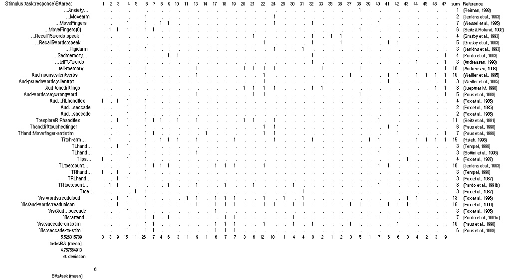
TABLE 1 LEGEND:
Table 1: Tabulation of 35 PET experiments (rows) x 38 Brodmann Areas (columns). Significant activation in a Brodmann Area is indicated by “1.” Experiments are encoded in three parts: stimulus;task;response. Experiments without stimuli lead with ellipses. Experiments without responses conclude with ellipses. Aud: auditory stimuli; T: tactile stimuli (R, L: right, left); Vis: visual stimuli. Other abbreviations are discussed in the figures below. For full details, see references.
The table shows that each Brodmann area is involved in an average of five tasks out of the thirty-five shown, or 14% of tasks. If all the experiments engaging a particular Brodmann area probed the same function, this observation would be compatible with isolating cognitive specialists, but inspection of Table 1 reveals that this is not the case. A few areas seem so far to be specialized, but the majority of them light up in scan after scan, and during very different cognitive and perceptual tasks. The busiest of them, Area 6, is engaged in 26 tasks, 74% of the various tasks listed. Meanwhile, the “specialists” (the six areas that activate for just one function) are not themselves the sole loci of their dedicated functions. Each specialized area is one part of a pattern involving, on average, nine other activated areas.
The case for distribution suggested by Table 1 is even stronger if one factors in the many steps of PET study design that favor localist interpretation, the assignment of “microfunctions” to regions of the brain. Foremost among these interpretive filters is the “subtraction method.” Each image is in fact a difference image, the result of a subtraction of a control condition from a test condition. Often the controls are components of the task. For example, to locate semantic processing the experimenters might use a control scan of subjects reading pseudowords, to isolate just the distinctive components of the task in question( Posner & Raichle, 1994). Even after this selective pre-screening of the data, however, the table shows distinct multifunctionality for most of the areas. Last but not least, the experiments indexed here are but a tiny slice of all the potential functions of the mind.
II. Visualizing distributed representation in the brain
If the reasoning in the previous section is correct, the localist claims must be severely hedged. For each conclusion of the form, “Subnet S computes function f,” we must substitute “Subnet S computes function f, among others.” This is not a trivial emendation. Cognitive neuroscience, if there is such a field, rests on the presupposition that we will ultimately discover bridge laws between the domains of cognitive psychology and neuroscience, particularly neurobiology. Elsewhere in physiology organs and organ systems have particular functions, and the job of science is to determine what these functions are. Localist interpretations of brain function fit into the traditional model, but distributed interpretations create a dilemma for cognitive neuroscience. The cognitive neuroscientist must choose between two midcourse corrections:
- Revise functional types: If the experimental evidence suggests that region R implements functions f1 or f2 or f3…, revisit that functional disjunction to see if there is a common factor to all of the disjuncts, where that common function is unique to R.
- Revise anatomical types: Seek a coherent way to describe the implementation level of cognitive functions that accounts for anatomically overlapping implementations of particular functions.
Lemma 1 forces a thorough revision of cognitive science, and with it the final abandonment of any realist interpretation of folk psychology or folk phenomenology. In its wake we would find ourselves describing our cognitive function in a language as yet unknown to us. (This prospect is welcomed by the Churchlands, for example( Churchland, 1986 , Churchland, 1989.) There is no reason not to embark on this long journey, and I do not see preemptive reasons why it must fail, although it might. It is the sole path only if Lemma 2 is shown to be incoherent. So, what about the second path, the revision of anatomical types? If the standard anatomy of Brodmann areas, not to mention gyri, sulci, and lobes — all the familiar station stops in the brain — are set aside (owing to their failure to map onto functional types), what possible new roadmap could we find?
The original champions of distributed processing, the connectionists, have faced just this issue. Many connectionist models feature hidden layers of neuron-like processing units in which localist interpretation breaks down. (Whence all the brouhaha about distributed processing.) In other words, the connectionists have faced a problem of interpreting processes controlled by large numbers of variables — a “multivariate” problem. So, when localism fails, connectionists turn to multivariate statistics for help, where one finds a fascinating variety of analytical techniques.
To illustrate a form of multivariate analysis, suppose we want to understand the various patterns of activation of a hidden layer of eighty units. That’s eighty variables, each with some role in determining the output of the network. Multivariate thinking begins with a conceptual shift: Regard each activation value as a magnitude along an axis or “dimension.” To start, the first variable, then, is a magnitude along the x axis, the second a magnitude along the y axis. The pair x,y accordingly can be represented, alá Descartes, as a point in “activation space.” With each additional variable, we add another axis at right angles to the previous axes. Eighty units, in this way of thinking, represent a space of eighty dimensions, a “hyperspace,” and the pattern of eighty activation values are interpreted as coordinates in that space. In other words, the pattern of activation with its eighty coordinates is reconceived as a singlepoint in 80-d space. It doesn’t matter that no such space could exist in our mundane reality, because it has the mathematical properties we will need. This 80-d space is thus a handy container for many patterns of activation — each reappears as a specific point in a high-dimensional map.
At this point the analysis proper begins: We can’t look at an 80- dimensional map, but we can measure its geometry. No matter how high the dimensionality, the notion of distance between points retains its usual non-boggling one-dimensional sense. Euclidean (linear) distance between any two points is easy to calculate, or one may calculate many other point-to-point relations with other algorithms. The result is a matrix of distances between points, not unlike a matrix of mileages between cities. What the matrix encodes, then, is some measure of similarity between each pair of points, or in other words, some measure of similarity between the multivariate patterns we started with. After this matrix has been constructed, one can represent the relations between points in several ways, each of which can reveal aspects of the structure of the galaxy of points in activation space. One appealing analysis of this type is multidimensional scaling (MDS) (The classic introduction is Kruskal & Wish, 1978 . A less formal introduction appears as an appendix in Clark, 1993 .) MDS uses the distance matrix from points in a high-d space to build a new mapping in a space of fewerdimensions. That is, MDS juggles the points on a map until it finds places for them that come as close as possible to preserving the inter-point distances. The MDS condensate can be of arbitrary dimensionality. In choosing the degree of shrinkage, however, one faces a tradeoff between accessibility and accuracy of the resulting low-d map. More dimensions afford a better fit between the new map and the actual distances, but remain hard to interpret, while fewer dimensions (two or three) are easy to visualize but, depending on the data, could be too procrustean, yielding a new map that wildly misplaces points. One sets the balance of accessibility and accuracy according to taste.
Let us suppose that our 80 units are each dedicated to just one function, in a completely localized, modular way; that is, each unit is active only when the network computes that function, and inactive otherwise. (For this example, assume that units are either on or off, 1 or 0 in activation value.) In that case, the 80-d activation space is studded with points that lie exactly on its 80 axes, each axis at right angles to all the others( 1,0,0…, 0,1,0…,0,0,1…, etc.). If we were to attempt MDS analysis of this space, we would encounter a double disappointment. First, as we shrunk the dimensionality of the space, we would be forcing points on orthogonal axes onto single new axes, resulting in a very bad fit, ever worse as the amount of shrinkage increases. Second, the activation space would be without structure. That is, every point is equidistant from every other. Any grouping of points will be completely arbitrary, not supported by underlying order in the space.
Now let us suppose that the hidden layer is a sparsely distributed processor. In this case, a subset of units work together to compute each function, and these subsets partially overlap from function to function. If we scale this space to fewer dimensions, the overlap means that axes can coalesce without as much forcing, and that the overlaps might reveal a meaningful structure in activation space. That is, where we judge two functions to be antecedently similar, we may expect the activation space to somehow reflect that similarity, and our new MDS’d map to reveal some of that structure. MDS can therefore serve as an indicator of distributed function. When a space shrinks into lower dimensions without excessive distortion (known in the MDS terminology as “stress”), that suggests distributed function.
Over the last two years I’ve been focusing the lens of MDS on the accumulated PET studies in Brainmap and in the PET literature in general. My goal has been to use MDS as a crude probe of brain activation space. If MDS works without excessive procrustean stress, and if the structures detected by MDS are meaningful, then this will offer another line of evidence that the brain is in fact a distributed processor.
As with any meta-analysis, this approach requires careful registration of the original experimental observations in a common format. The PET studies themselves already encourage comparisons in many ways. Individual brains differ strikingly in size and shape, so a routine part of PET processing is the morphing of one’s personal brain into the shape of a standard brain, so that points of activation can be localized to comparable anatomical structures. In addition, PET studies always involve multiple subjects. The resulting patterns of activation are averaged (and peaks tested for significance), washing out stray activations, whether due to idiosyncrasy or to a subject’s drifting off the task. Beyond that, however, the studies differ from each other in one important way: As mentioned above, the reported patterns of activation are generally “difference images,” created by subtracting a baseline or control pattern from the test or task pattern. These baseline controls are not uniform in the literature. For example, in a study of semantic processing, study A might image a brain during reading aloud, and subtract from that a control task consisting of reciting the alphabet. The point of this subtraction would be to isolate the subsystem involved in processing word meaning, while factoring out that involved in simple vocalizing. Study B, meanwhile, might also image a brain during reading aloud — the same test task — but subtract from it a control task consisting of reading silently. In this case, the function of interest is vocalizing itself. Both studies might display patterns of activation labelled “reading aloud,” and indeed the underlying activation in the brains involved might be very similar, but the divergent subtracted control states would yield divergent difference images.
As a result, any PET meta-analysis must rest on a collection of experiments that share a common control state. There are a few such familiar baselines in the literature. One of the most common baselines is simple rest with closed eyes. A full review of hundreds of PET papers yielded 36 experiments where the difference image was based on a control state where subjects rested quietly with eyes closed. These are the same experiments listed (with their bibliograpic references) in Table 1. (Another common control condition has open-eyed subjects focus on a fixation point on a blank screen. This will be reviewed in a future study.) In these 36 experiments, points of activation were assigned using a brain atlas (as well as published anatomical assignments) to 87 cortical and subcortical sites. [NOTE: The smallest sites were the Brodmann areas. Others included cortical gyri and sulci and major subcortical cerebral structures. The largest regions were the four major cerebral lobes. Overlapping regions and double-counted activations were tolerated in order to maximize the chances of detecting activity in any and all functionally overlapping areas. For similar reasons, the right and left hemispheres were superposed On the one hand, this superposition may have obscured some functional differences between hemispheres. But on the other hand, the superposition eliminated a spurious separation of patterns due to spatial and bodily location. A tactile stimulus to the right hand should be comparable to the same stimulus delivered to the left hand, despite the differences in laterality in the sensory cortex. END OF NOTE] To wax multivariate, individual patterns of activation in the brain were conceived as points in an 87 dimensional space. From here, multidimensional scaling generated maps in fewer dimensions. Surprisingly, the procrustean stress, or badness of fit, was quite low even when the hyperspace was squeezed into 3 dimensions. (Stress = .13. Stress values under .2 are considered “good fits.” See Kruskal & Wish, 1978 ).[NOTE: There is no standard test for statistical significance in MDS. I probed significance by generating five random sets of thirty six vectors with statistical properties similar to the PET data. The MDS process found solutions for the random patterns with a mean stress of .246, standard deviation .006. Five different MDS runs on the PET data yielded a mean stress of .137, standard deviation .005. These differences are significant, p<.0001.END OF NOTE]
Even without interpretation, the successful shrinkage of hyperspace implies distributed function, as argued above. But, in addition, MDS revealed the crude outlines of the structure of brain activation space. The largest regional affinities in brain space were determined by the modality of input. Tactile, visual, and auditory conditions tended to group. The groupings were not compact clusters, however, but rather rough ellipsoids. In other words, in many cases similarity of input modality leads to collinearity of resulting points in brain activation space. Within the modalities, there is some indication of further structure, and this seems to be in part a reflection of the response made to the various tasks in the map.
The figures below reveal this internal structure. Each is a view through a 3-dimensional MDS space, based on the 36 experimental points in 87 dimensions. In the figures, only the relative position of points is meaningful; The XYZ axes are arbitrary. Nor do the positions of points bear any one-to-one relationship with anatomical or physical points in the brain. Each point represents an activation pattern of ten or more anatomical components, and point proximity indicates similarity among patterns.
Graphically, each figure is an “exploded” three dimensional map. Data points appear twice, once in their correct location in the scaled space, reflecting their true degree of similarity, and then again as they would project onto a sphere. The “real” point and its projection onto the sphere are connected by a dotted line. The spherical projections (along a ray from the origin to the surface of the sphere) identify regions of brain space shared by groups. Nearness of points on the surface of the sphere no longer indicates absolute similarity, but corresponds to the closeness of points to a line radiating from the origin. More important, regions of the sphere as defined by collections of data points correspond to regions in brain space. Each is a slice of a three-dimensional pie, a wedge or cone radiating from the xyz origin. Thus the “continents” of this new found land arise from the underlying order of points.
In short, the images that follow condense a large quantity of data — many experiments, many subjects. Here then is a first multivariate survey of “brain activation space,” and a brain-based window into the mind. Figure 1. Overview of MDS space. The “icecap” is designated north for ease of reference. Eighteen of thirty-six data points are shown. The points seem to fall in three rough groups. Most of the projected points lie near a great circle, indicating that this set of points is approximately coplanar. The groups themselves are roughly elliptical.

Figure 2. Audition. The “north pole” projects from a group of auditory tasks. It seems to make little difference whether the sound is produced by the subject or not. The tasks encoded: Recall (aloud) a five word list heard prior to the scan; recall (aloud) a fifteen word list heard prior to the scan; Listen to and silently repeat a pseudoword list; Listen to verbs and speak an associated pronoun (from a list of pairs learned prior to the scan); Say words beginning with “C”; Listen to verbs and speak the pronoun notassociated, contradicting a list of pairs learned prior to the scan; Lift index fingers in time to a metronome; Silently produce verbs appropriate to heard nouns; and tell a remembered incident. From the spherical projections and proximities of points, it can be seen that the northern points are approximately collinear. Verbal response tasks seem to collect toward the top of the line.
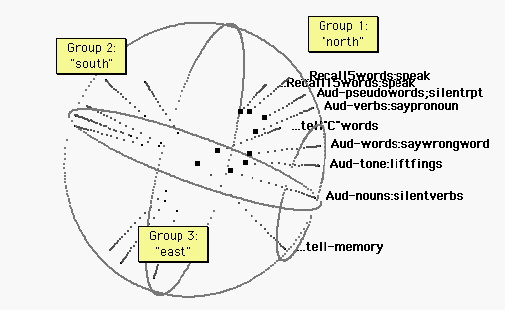
Figure 3. Vision and auditorily cued tasks. The sphere has been rotated for legibility. The “east pole” includes repetitive tasks timed to a metronome. (See figures 4 and 5.) The south pole is the realm of visual cognition. Tasks include: Read a text in unison with others; Read a text aloud; Saccade between two alternately flashing light sources; saccade between two light sources in time with a metronome; saccade to a light source that might appear anywhere; watch for a light (which does not appear.) Language tasks group at one end of the visual ellipsoid. The auditory ellipsoid (figure 2) and the visual ellipsoid below are similar in orientation, and the verbal response tasks group at approximately the same end of each ellipsoid.
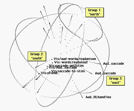
Figure 4. Eighteen other tasks. “East” is indicated by projections of the three auditorily cued tasks depicted in figure 3. Several of the remaining eighteen tasks are also”easterly.” However, the poles of vision and audition are not occupied by these nonvisual and nonauditory tasks.
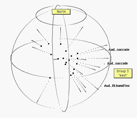
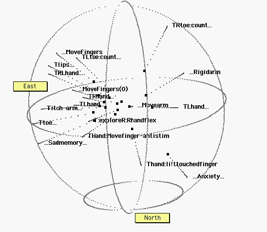
Figure 5. Tactile, motor, and no-stimulus tasks. The sphere has been rotated for ease of interpretation, revealing a broad “equatorial” band of tactile (T) tasks. R, L: Right, Left. Ellipses (…) indicate no stimulus (at the beginning of a label) or no response (at the end of a label). Some specific tasks: Titch-arm: an itch on the arm.;…Sadmemory…: Subjects ruminated on a sad event; …Anxiety…: Subjects waited for a painful electric shock (which never came). Within this region, there is no obvious further organization.
III. Terra cognita.
The figures above suggest that brain space is organized into regions. Two of these, occupied by visual and auditory perception tasks, form ellipsoidal regions with rough axes reflecting the commonalities among a group of tasks (=collinearity or proximity) as well as organizing their differences (=placement along the axis). But one would like to know how the overall space is arranged. That is, how are the axes related to each other? To visualize this structure is to visualize terra cognita. Figure 6 depicts all 36 tasks, by their groups.
Figure 6. All thirty six points.X: tactile, motor, and proprioceptive tasks; Y: auditory tasks, or auditorily cued tasks. Z: visual tasks. Despite some exceptions, these three types of tasks tend to occupy distinct regions in brain hyperspace. Notwithstanding the noise in the data, and the distortions (stresses) in the representation, it appears that the distance senses generally fall on a north-south axis. In contrast, the bodily senses, including proprioceptive motor feedback, distribute around a broad equatorial band. These bodily tasks appear to require at least one additional dimension, compared to the distance senses.
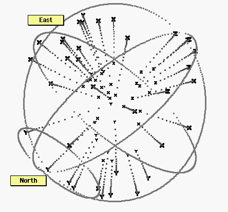
Among the auditory stimuli tasks are three located near the “east pole.” As it happens, these tasks included a significant motor component: In two of these tasks, subjects looked back and forth between targets, in one case two lights, in the other the remembered locations of previous lights. The auditory cue was a metronome that set a rhythm for the back-and-forth saccadic eye movements. The other outlying task involves a hand motion cued by a tone. It makes sense that these would be mapped among other motor tasks.
Reviewing the spheres, we find the following rough geography:
- “North pole”: the auditory world
- “Equatorial regions”: the tactile, proprioceptive, and motor world
- “South pole”: the visual world
The spherical projection suggests the large-scale structure of “brain activation space,” while the various MDS figures reveal groupings and structure for subsets of the MDS’d data points. Brain space, in short, seems to exhibit both global and local structure.
IV. Toward interpretation
The main question of this paper is empirical: Is the brain a distributed processor (probably sparsely distributed), or is it an assembly of local processors (probably implemented in dedicated networks)? The argument for distribution unfolded in two parts: In the first, a large-scale comparison of PET experiments was shown to suggest multi-functionality for many Brodmann areas, a result which is inconsistent with localism. In the second, the measurable success of multidimensional scaling showed the brain as a distributed processor. The 87 dimensions of the patterns of activation shrank (via multi-dimensional scaling) smoothly into a 3-dimensional map. Since the hyperspace of local processors would resist shrinkage, this result strongly suggests an underlying order of distributed processors.
These results are subject to the uncertainties that bedevil any meta-analysis. Different experiments use different protocols, different (and usually small) subject populations, different statistical filters, and different scanning instruments. With the help of dedicated students and collegial experts, I have been grappling with these confounds, and will continue to revise the approach. Despite the low resolution and noise affecting the MDS analysis, I feel increasingly confident that the analysis is imaging a true distributed processor, rather than an artifact of my approach.
So far, so good. The next level of observation calls for quite a bit more interpretation. In addition to being mappable, brain activation space “made sense.” Tasks that seem similar seem to fall near one another, and certain big distinctions we make, e.g., between the senses, make an appearance on the map. At first glance, this result seems almost trivial: Since the various tasks resemble one another in various ways, it makes sense that even a fancy multivariate analysis would simply give back those resemblances, now translated into distances on a map. This inevitability is an illusion, however. Resemblances in task descriptions played no role in the MDS analysis, which derived entirely from brain activity. Rather, the analysis levelled the field, treating all brain areas as equal and making no assumptions about the relation of any area, or any pattern of areas, to a task. That is, the patterns of brain activity could have been organized in myriad ways that would not make sense, or would make less sense than this. This implies that the way we organize “task space,” deriving from whatever mix of folk psychology, retrospection, and cognitive science, is quite similar to the way the brain organizes itself. “Task space” reflects our psychology, but it also is the space of the brain. Thus, the map is in fact two maps. Their isomorphism (such as it is) suggests that the tasks and functions psychology appeals to are biologically real, that our self knowledge (such as it is) is genuine. Mind is brain — that is old news. But that the particular expressions of mind can be hooked into particular states of the brain, and that the overall structure of mentality and the overall structure of the biggest known neural net should more-or-less coincide, this is progress.
The next steps are progressively more wobbly. The end-point and goal of multi dimensional scaling is to discover a limited number of dimensions that offer a compact representation of the initial high-dimensional domain. Three dimensions are a great improvement over eighty seven, but thirty six points are still a crowd. An important part of the next phase of interpretation is visualization. As the figures suggest, the interpreter here faces many choices. In general, one can consider any and all subsets of the thirty five, thinking globally or locally. As a result, the search for interesting relationships balloons toward epic proportions.
Humbled by an awareness that the quest could be interminable, nonetheless we can ponder some suggestions for interpretation, ranging from large scale to small. As the first tourists to this particular scenic overlook, we’ll briefly consider a few exemplary issues.
Q: The geography of Planet Brain roughly separates points according to the modality of the input. But do the relative positions of the three main “continents” mean anything?
A: We can look at the big divisions between regions, or we can look at polar opposites, asking in both cases, is there a difference? The northern hemisphere tasks tend to be verbal, and the southern tasks tend to be spatial — with two conspicuous exceptions, both involving reading aloud. Alternatively, one could look at distinctions in the kind of processing required by various tasks. In this case, the southern tasks all require the translation of a two-dimensional receptor array (the retina, cutaneous receptors) into a 3 dimensional spatial representation of objects (including words) in space and bodily posture and location. The northern tasks involve far less of this world-building. For most of them, stimulus location and posture play no role in the task. Instead the stimuli are mere cues (or the task is uncued), and the task is experienced as interior, in contrast to the exteriorized south.
Q: Within the modalities of sight and hearing, the maps seem to show collinearity of points. What is the meaning of that? Why are they not in tight clumps instead?
A: Tasks at the opposing poles of these ellipsoid regions are maximally distinct in brain space. They are, from the brain’s point of view, very different tasks. A tight clumping would ignore these distinctions. On the other hand, tasks sharing a kind of stimulus each have something in common too, and brain space captures that in the simplest way that represents both their differences and similarities, by lining them up. If they were clumped, in brain space they would all be indistinguishable tasks. If they were scattered with no order at all, then the map (and the underlying space) would not reflect the similarities within each group.
Q: What about that equatorial band? It seems so disorganized, compared to the visual and auditory world.
A: “Disorganization” suggests that additional dimensions are needed to organize this region of brain space, a hypothesis that could be explored by performing separate MDS analyses on subsets of the data. The question can be posed at the cognitive level, too: Is the space of the bodily senses more complex than the space of the distance senses? It is in at least the following way: To build a perceptual world from tactile and proprioceptive stimuli, one must coordinate two distinct streams of information, the inputs from the cutaneous receptors and the proprioceptive receptors. That is, the bodily senses are unique in that the sensory array is constantly changing shape, and the convolution of the limbs and torso must be factored in with the sensory stream to construct a tactile world of solids. Ears and eyes are fixed in relative location, and so those senses have the relatively simpler task of tracking change of viewpoint over time. It appears that this relative simplicity appears in the multivariate analyses presented here.
Even these three sketchy forays suggest the open-endedness of interpretive opportunities here. It will require many more expeditions to terra cognita to discover its organizing principles, and it will require a more rigorous examination of “task space” than I have provided, before we can confidently read the mind in the brain, the brain in the mind. Still, notwithstanding the fuzzy images, it appears that the multivariate lens, held to a distributed neural processor, suggests a brain not unlike the mind we supposed that we had. Thus encouraged, we might launch further, more exacting probes into inner space. The ever-expanding meta-analysis of functional brain images might show us the extent to which our phenomenology reflects the real order of the brain. We may one day see the mind not only from our own subjective and culture-bound points of view, but from the point of view of the brain itself.
Acknowledgements: Thanks to David Herman, Julie Guilbert, Kate Weingartner, Heather McAleer, Alison Rada, Patricia Park-Li, Jeffrey Harris, Tanya Suvarnasorn, Elizabeth Worthy, and Claudine Bitel for their help in compiling the PET data. This work was supported by a Faculty Research Grant from Trinity College.
REFERENCES
Andreasen, N. (1998). Remembering the past: two facets of episodic memory explored with positron emission tomography. American Journal of Psychiatry, 152, 1576-1585.
Bottini, G., Paulesu, E., Sterzi, R., Warburton, E., Wise, R., Vallar, G., Frackowiak, R., & Frith, C. (1995). Modulation of conscious experience by peripheral sensory stimuli. Nature, 376, 778-781.
Churchland, P. (1989). A Neurocomputational Perspective. Cambridge, MA: MIT Press.
Churchland, P.S. (1986). Neurophilosophy: Toward a Unified Sceince of the Mind/Brain. Cambridge, MA: MIT Press.
Clark, A. (1993). Sensory Qualities. Oxford:: Clarendon Press.
Dupont, P., Orban, G., Vogels, R., Bormans, G., Nuyts, J., Schiepers, C., De Roo, M., & Mortelmans, L. (1993). Different perceptual tasks performed with the same visual stimulus attribute activate different regions of the human brain: A positron emission tomography study. Proceedings of the National Academy of the Sciences, 90, 10927-10931.
Fox, P., Fox, J., Raichle, M., & Burde, R. (1985). The role of cerebral cortex in the generation of voluntary saccades: a positron emission tomographic study. Journal of Neurophysiology, 54(2), 348-369.
Fox, P., Burton, H., & Raichle, M. (1987). Mapping human somatosensory cortex with positron emission tomography. Journal of Neurosurgery, 67, 34-43.
Fox, P., Ingham, R., Ingham, J., Hirsch, T., Downs, J., Martin, C., Jerabek, P., Glass, T., & Lancaster, J. (1996). A PET study of the neural systems of stuttering. Nature, 382, 158-162.
Grasby, P., Frith, C., Friston, K., Bench, C., Frackowiak, R., & Dolan, R. (1993). Functional mapping of brain areas implicated in auditory-verbal memory function. Brain, 116, 1-20.
Howard, D., Patterson, K., Wise, R., Brown, W., Friston, K., Weiller, C., & Frackowiak, R. (1992). The cortical localization of the lexicons. Brain, 115, 1769-1782.
Hsieh, J. (1998). Urge to scratch represented in the human cerebral cortex during itch. Journal of Neurophysiology, 72, 3004-3008.
Jenkins, I., Bain, P., Colebatch, J., Thompson, P., Findley, L., Frackowiak, R., Marsden, C., & Brooks, D. (1993). A positron emission tomography study of essential tremor: Evidence for overactivity of cerebellar connections. Annals of Neurology, 34, 82-90.
Jueptner M, (1998). Localization of a cerebellar timing process using PET. Neurology, 45, 1540-1545.
Kruskal, J. & Wish, M. (1978). Multidimensional Scaling. Beverly Hills, CA: Sage.
Lueck, C., Zeki, S., Friston, K., Deiber, M., Cope, P., Cunningham, V., Lammertsma, A., Kennard, C., & Frackowiak, R. (1989). The colour centre in the cerebral cortex of man. Nature, 340, 386-389.
McClelland, J. & Rumelhart, D. (1986). Parallel Distributed Processing: Explorations in the Microstructure of Cognition. Volume Two: Psychological and Biological Models. Cambridge, MA: MIT Press.
Pardo, J., Raichle, M., & Fox, P. (1991a). Localization of a human system for sustained attention by positron emission tomography. Nature, 349, 61-63.
Pardo, J., Raichle, M., & Fox, P. (1991b). Localization of a human system for sustained attention by positron emission tomography. Nature, 349, 61-63.
Pardo, J., Pardo, P., & Raichle, M. (1993). Neural correlates of self-induced dysphoria. American Journal of Psychiatry, 150, 713-719.
Paus, T., Petrides, M., Evans, A., & Meyer, E. (1998). Role of the human anterior cingulate cortex in the control of oculomotor, manual and speech responses: a positron emission tomography study. Journal of Neurophysiology, 70, 453-469.
Petersen, S., Fox, P., Posner, M., Mintun, M., & Raichle, M. (1988). Positron emission tomographic studies of the cortical anatomy of single-word processing. Nature, 311, 585-589.
Posner, M. & Raichle, M. (1994). Images of Mind. San Francisco, CA:: Scientific American Press.
Reiman, E. (1998). Neuroanatomical correlates of anticipatory anxiety. Science, 243, 1071-1074.
Rumelhart, D. & McClelland, J. (1986). Parallel Distributed Processing: Explorations in the Microstructure of Cognition. Volume 1: Foundations. Cambridge, MA: MIT Press.
Seitz, R., Roland, P., Bohm, C., Greitz, T., & Stone-Elander, S. (1991). Somatosensory discrimination of shape: tactile exploration and cerebral activation. European Journal of Neuroscience, 3, 481-492.
Seitz, R. & Roland, P. (1992). Learning of sequential finger movements in man: a combined kinematic and positron emission tomography (PET) study. European Journal of Neuroscience, 4, 154-165.
Tempel, L. (1998). Abnormal cortical responses in patients with writer’s cramp. Neurology, 43, 2252-2257.
Weiller, C., Isensee, C., Rijntjes, M., Huber, W., Mueller, S., Bier, D., Dutschka, K., Woods, R., Noth, J., & Diener, H. (1995). Recovery from Wernicke’s aphasia: a positron emission tomographic study. Annals of Neurology, 37, 723-732.
Wessel, K., Zeffiro, T., Lou, J., Toro, C., & Hallett, M. (1995). Regional cerebral blood flow during a self-paced sequential finger opposition task in patients with cerebellar degeneration. Brain, 118, 379-393.
Zeki, S., Watson, J., Lueck, C., Friston, K., Kennard, C., & Frackowiak, R. (1991). A direct demonstration of functional specialization in human visual cortex. The Journal of Neuroscience, 11, 641-649.
Reiman, 1998
Jenkins et al., 1993
Wessel et al., 1995
Seitz & Roland, 1992
Grasby et al., 1993
Grasby et al., 1993
Jenkins et al., 1993
Pardo et al., 1993
Andreasen, 1998
Andreasen, 1998
Weiller et al., 1995
Weiller et al., 1995
Jueptner M, 1998
Paus et al., 1998
Fox et al., 1985
Fox et al., 1985
Fox et al., 1985
Seitz et al., 1991
Paus et al., 1998
Paus et al., 1998
Hsieh, 1998
Tempel, 1998
Bottini et al., 1995
Fox et al., 1987
Jenkins et al., 1993
Tempel, 1998
Fox et al., 1987
Pardo et al., 1991a
Fox et al., 1987
Fox et al., 1996
Fox et al., 1996
Fox et al., 1985
Pardo et al., 1991b
Paus et al., 1998
Paus et al., 1998
Petersen et al., 1988
Dupont et al., 1993
Pardo et al., 1991b
Zeki et al., 1991
Howard et al., 1992
Lueck et al., 1989