
I chose to have 2500 tweets in my data set with all those tweets coming from March 8th – March 9th. I chose 2500 tweets because we were recommended to have a subset data set of tweets between 2000-3000 tweets and I thought that 2500 tweets would be a good sample size. The time period I chose really had no significance; my data set ended on March 9th and to make things run smoother, I just used the first 2500 tweets I had. I have a total of 3524 tweets in my new file. I believe that some columns on the right are blank because some tweets didn’t mention anybody in them or on the other hand, mentioned more than one person.
There are a total of 77 nodes and 254 edges in the file.
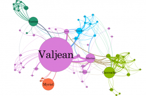
I chose undirected because it shows all the different mutual relationships in the data file. Undirected graph is able to display connections between people in a better way when compared to directed graphs.
Valjean has ID number 11. Fantine has ID number 23. Valjean is connected to four targets with ID numbers 0, 2, 3 and 10 while Fantine is connected to nine targets with ID numbers 11, 12, 16, 17, 18, 19, 20, 21 and 22. Although Valjean is the main character, Fantine had just over double the amount of target connections that Valjean had. Based on this data, I believe that Fantine is the main source.
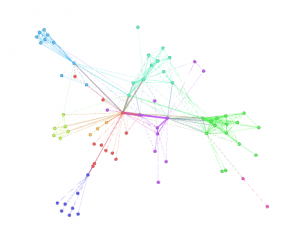
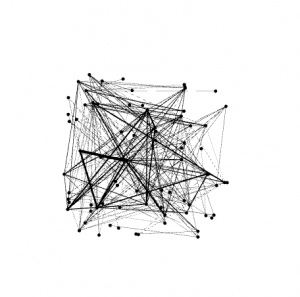
For some reason, when I increased the repulsion strength, my graph became colorful, but not as messy and disorganized. When I increased the repulsion strength, I think that my graph narrowed down all the connections to the connections that are seen most frequently on Twitter. The most frequent interactions are now shown in the graph above, whereas they were not shown in the first graph.
Average path length = 2.6411483253588517 Diameter = 5
When I picked Betweenness Centrality and set the minimum size to 10 and maximum size to 200, the size of each node changed. What I think happened is that the larger the node, the more connections that node has whereas the smaller the node, the less connections that node has (I could be 100% wrong).
PART III:
The repulsion strength I chose was 10,000 because I was advised to do so by Professor Gieseking. My average path length was 5.016561091911934 and diameter was 16. This means that most relationships are 19 connections apart and separated by 6.732 degrees of diameter.
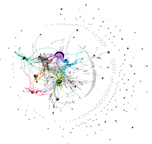
The largest nodes in my graph were “POTUS” and “speakerryan”. What I find interesting about this was that POTUS and speakerryan were both the largest words in my word cloud we created in lab three. This makes sense as many people are tweeting at the president of the United States, Donald Trump, as his goal is to repeal Obamacare; this would negatively impact a majority of people in America as they depend heavily on Obamacare for health insurance and medical expenses. Speakerryan was a large node too which makes sense as he’s heavily involved in this whole process of repealing Obamacare and coming up with a new plan. Interestingly enough, POTUS and speakerryan were separated whereas I thought that they would be more connected.
I expected many of the big government figures to be connected, but like I said above, they don’t seem to be very connected, meaning they don’t communicate too often on Twitter. I feel like POTUS was the largest node as so many people are against President Trump and his new theories/policies. The dates of the tweets I used in my dataset were from March 8th- March 9th, but many huge things have happened involving Obamacare in the last week and a half, which kind of makes the time period of this data not very helpful. In the last week, it was decided that Obamacare was not going to be repealed, but unfortunately, I stopped collecting tweets on Obamacare. I think that the singletons reveal that people may be talking about Obamacare, but not talking in the same conversations that the people in color are talking in (different context).
Hi Danny. I found it very interesting that the largest nodes in your graph are “POTUS” and “speakerryan” because your hashtag is in fact #obamacare. I was also as surprised as you seem to be about the graph not showing as many powerful political figures as you assumed there to be. Since President Donald Trump uses Twitter as a daily form of communication, you would think that most political figures would use it as well. However, this graph helps us understand that not all politicians see Twitter as a useful form of communication.
Something to consider for your next lab is to make the photographs you add into the post a higher resolution. I cannot zoom into the photo of your Gephi to see the details of the nodes. You can solve this problem by adding the attachment as high resolution.
You did a nice job of comparing lab 3 in your post for lab 4, and makes me think that I should have done a better job pointing out the similarities between the two labs and talk about how each set of data I found in each relate to one another.
Danny, this is yet again another great post. Firstly, I found it interesting how connected your graph looked. The graphs you and Katherine have both look completely different from mine which is something I found fascinating. I also found it interesting that therealdonaldtrump did not have a larger node because I know Donald Trump tends to tweet from his personal account. I agree with you because I too would have expected for more political leaders to be connected. I enjoyed how you connected your lab 3 and lab 4. This is something I wish I had done. I wish that you had looked up the tweets from some of your accounts because it could have added to the picture of your graph.